Spread.NET 14 WinForms includes support for two important Excel calculation functions: XLOOKUP and XMATCH. These new functions are recent additions to Excel.
XLOOKUP
The XLOOKUP function performs a lookup on the specified lookup_value in the specified lookup_array using the specified match_mode and search_mode, and then returns a value from the corresponding cell in the specified return_array.
XLookUp syntax

The XLOOKUP function is a new lookup function which can replace the old LOOKUP, VLOOKUP, and HLOOKUP functions. The new function is better for several reasons:
- XLOOKUP can perform vertical or horizontal lookups (or both when nested), depending on the orientation of lookup_array.
- XLOOKUP can perform non-exact lookups with correct results, even when the data is not sorted (unlike HLOOKUP/VLOOKUP).
- XLOOKUP does not require referencing the entire range containing lookup_array and return_array, only those two particular ranges – thus XLOOKUP can be more efficient in terms of required recalculations.
- XLOOKUP arguments adjust automatically when columns or rows are inserted or removed that move the lookup_array and return_array, since it used range references instead of indexes.
- XLOOKUP can return 0 or some other useful value instead of #N/A when you specify the if_not_found argument.
- XLOOKUP is enhanced in Spread. NET 14 WinForms to support a new search_mode 0 - All which returns all matching items in an array. It can spill to adjacent cells when dynamic arrays are enabled.
Download a trial of Spread.NET today!
To illustrate the XLOOKUP function in action, here is a sample table named XLookupData1:

Example 1 shows the most typical use case, the vertical lookup using exact match:

The XLOOKUP function searches for lookup_value (7) inside the lookup_array (XLookupData1[Number]) and returns the corresponding value from the return_array (XLookupData1[English]) using this formula:
=XLOOKUP(H20,XLookupData1[Number],XLookupData1[English])
The other formulas work similarly, returning values from the French and Spanish columns, respectively:
=XLOOKUP(H20,XLookupData1[Number],XLookupData1[French])
=XLOOKUP(H20,XLookupData1[Number],XLookupData1[Spanish])
Note that, unlike VLOOKUP, the default behavior of XLOOKUP performs the search using match_mode 0 - exact match and search_mode 1 - first to last when those arguments are not specified.
Example 2 shows how XLOOKUP can perform a lookup that returns a value that is to the left or above the lookup_array. VLOOKUP and HLOOKUP cannot do this:

Example 2 uses XLOOKUP to search the Spanish column for the specified word in cell C33 and return the corresponding values from the Number, English, and French columns:
=XLOOKUP(C33,XLookupData1[Spanish],XLookupData1[Number])
=XLOOKUP(C33,XLookupData1[Spanish],XLookupData1[English])
=XLOOKUP(C33,XLookupData1[Spanish],XLookupData1[French])
The next example uses the transpose of the XLookupData1 table to demonstrate horizontal a lookup:

Example 3 shows how XLOOKUP can perform a horizontal lookup by referencing a horizontal range for lookup_array:

Example 3 uses XLOOKUP to search the Number row for the specified value in C46 and return the corresponding values from the English, French, and Spanish rows:
=XLOOKUP(C46,C40:L40,C41:L41)
=XLOOKUP(C46,C40:L40,C42:L42)
=XLOOKUP(C46,C40:L40,C43:L43)
This is identical to Example 1, except that the search is performed horizontally because the table is transposed.
Example 4 shows how XLOOKUP can perform a horizontal lookup and return items from rows that are above the lookup_array range:

Example 4 uses XLOOKUP to search the Spanish row for the specified value in I46 and return the corresponding values from the Number, English, and French rows:
=XLOOKUP(I46, C43:L43,C40:L40)
=XLOOKUP(I46, C43:L43,C41:L41)
=XLOOKUP(I46, C43:L43,C42:L42)
This is identical to Example 2, except that the search is performed horizontally because the table is transposed.
The next example uses the following table XLookupData3, a typical table listing commission rates:

Example 5 shows how XLOOKUP can perform a search and return exact match or next smaller value:

Example 5 uses XLOOKUP to search the Sales column for the specified value in F58 using match_mode -1 - exact match or next smaller value:
=XLOOKUP(F58,XLookupData3[Sales],XLookupData3[Commission],,-1)
The next formula is identical, except for the addition of the search_mode argument specifying 2 - binary search on ascending lookup_array.. This is faster when the table is sorted, as in this case:
=XLOOKUP(F58,XLookupData3[Sales],XLookupData3[Commission],,-1,2)
The legacy LOOKUP function can also work to find the rate in the sorted table. Since the table is organized with the lookup_array in the first column and the return_array in the last column, the formula is actually much simpler:
=LOOKUP(F58,XLookupData3)
The legacy LOOKUP function also supports specifying the lookup_array and return_array separately, like XLOOKUP:
=LOOKUP(F58,XLookupData3[Sales],XLookupData3[Commission])
The VLOOKUP function can also do this:
=VLOOKUP(F58,XLookupData3,2)
However, when the XLookupData3 table is sorted in reverse order:

Then, all the other formulas break and return the wrong result, except for the first formula using XLOOKUP:

The next example uses the following table XLookupData4, listing various maximum numbers of units that can fit in particular sized boxes:

Example 6 show how XLOOKUP can perform a search and return exact match or next larger:

Example 6 uses XLOOKUP to search the Units column for the value in F70 using match_mode 1 - exact match or next larger to find the appropriate box size:
=XLOOKUP(F70,XLookupData4[Units],XLookupData4[Box Size],,1)
The next example uses the following table XLookupData5. This table lists chess openings and associated moves:

Example 7 shows how XLOOKUP can perform a search using match_mode 2 - wildcard match:

Example 7 uses XLOOKUP to search the Name column for the value in G77 using match_mode 2 - wilcard match to find the associated ECO and Move(s):
=XLOOKUP(""&G77&"",XLookupData5[Name],XLookupData5[ECO],,2)
=XLOOKUP(""&G77&"",XLookupData5[Name],XLookupData5[Move(s)],,2)
Wildcard match uses '?' to represent any character and '*' to represent any sequence of characters. It applies only when match_mode 2 - wildcard match is specified.
The next example uses the following table XLookupData6. This table lists the start date, name, and department of people, which contains some duplicates:

The duplicate entries in the table represent people who have switched to a different department from a reorganization.
Example 8 shows how XLOOKUP can perform a search and return the last matching item:

Example 8 uses XLOOKUP to search the Name column for the value in G87 using search_mode -1 - last to first:
=XLOOKUP(G87,XLookupData6[Name],XLookupData6[Dept],,,-1)
Returning the last item will depend on the current order of the items in the table.
XLOOKUP can also reference a range of cells or a spilled array reference for the lookup_value argument, and spill results when dynamic arrays are enabled:

In the above example, cell F90 contains a dynamic array formula which spills results to F90:F97:
=SORT(UNIQUE(XLookupData6[Names]))
The formula in the cell G90 uses XLOOKUP with lookup_value F90# and spills results to G90:G97:
=XLOOKUP(F90#,XLookupData6[Name],XLookupData6[Dept],,,-1)
The legacy LOOKUP function can also do this:

However, the LOOKUP function requires this complex array formula to return the correct result – here is the formula in cell P90:
=LOOKUP(2,1/(XLookupData6[Name]=O90),XLookupData6[Dept])
That formula is a tricky way to get the desired result. First, the lookup_value specified (2) is deliberately chosen so that no match will be found. Then, the second argument specifies 1/(XLookupData6[Name]=O90, which first evaluates the array formula part (XLookupData6[Name]=O90) to an array of True (1) and False (0) values. This specifies whether or not the particular cell in XLookupData6[Name] is equal to the specified name in O90. Then, each element is divided into 1, which results in a new array of values. It contains True (1) for each name equal to the value in O90 and #DIV/0 error values, where the previous array contained False (0) values.
The LOOKUP function will not find the lookup_value (2) in any of those array elements (by design), and it returns the value associated with the last non-error value in the array.
The formula using LOOKUP is not only more complicated, but also cannot work using a range or dynamic array argument (e.g., using O90# instead) because LOOKUP does not support dynamic arrays or spilling behavior. Instead, the formulas in the cells P91:P97 must be copied down from P90.
Example 9 shows how XLOOKUP can perform a search using search_mode 0 - all and return all the matching elements in a dynamic array:

Example 9 uses XLOOKUP to search the Name column for the value in C101 using search_mode 0 - all:
=XLOOKUP(C101,XLookupData6[Name],XLookupData6[Start],,,0)
=XLOOKUP(C101,XLookupData6[Name],XLookupData6[Dept],,,0)
The first formula in B103 finds the start dates for Fred, and the second formula in C103 finds the associated Dept.
Note that this search_mode 0 - all is unique to Spread.NET and not supported in Excel (which will return a #VALUE! error).
XMATCH
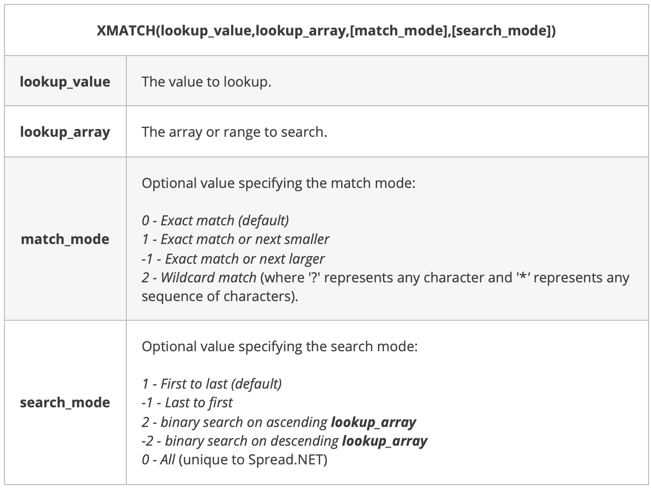
XMatch syntax
The XMATCH function performs a lookup on the specified lookup_value in the specified lookup_array using the specified match_mode and search_mode, and then returns the index of the found item in lookup_array.
The XMATCH function is a new lookup function which can replace the old MATCH function. The new function is better for several reasons:
- XMATCH can perform vertical or horizontal lookups (or both when nested), depending on the orientation of lookup_array.
- XMATCH can perform non-exact lookups with correct results, even when the data is not sorted (unlike MATCH).
- XMATCH is enhanced in Spread .NET 14 WinForms to support a new search_mode 0 - All. It returns all matching items in an array, which can spill to adjacent cells when dynamic arrays are enabled.
To illustrate the XMATCH function in action, here is a sample table named XMatchData1:

Example 1 shows the most typical use case, the vertical lookup using exact match:

The XMATCH function in H20 searches for lookup_value (7) inside the lookup_array (XMatchData1[Number]), and returns the index in lookup_array using this formula:
=XMATCH(H20,XMatchData1[Number])
The MATCH function in H23 does the same:
=MATCH(H19,XMatchData1[Number])
The next example uses the transpose of the XMatchData1 table to demonstrate horizontal a lookup:

Example 2 shows how XMATCH can perform a horizontal lookup by referencing a horizontal range for lookup_array:

Example 2 uses XMATCH to search the Number row for the specified value in C38 and return the index:
=XMATCH(C38,C32:L32)
The MATCH function in C42 does the same:
=MATCH(C38,C32:L32)
The next example uses the following table XMatchData3, a typical table listing commission rates:

Example 3 shows how XMATCH can perform a search and return exact match or next smaller value:

Example 3 uses XMATCH in F49 to search the Sales column for the specified value in F48 using match_mode -1 - exact match or next smaller value:
=XMATCH(F48,XMatchData3[Sales],-1)
The next formula in F50 is identical, except for the addition of the search_mode argument specifying 2 - binary search on ascending lookup_array. This is faster when the table is sorted, as in this case:
=XMATCH(F48,XMatchData3[Sales],-1,2)
The legacy MATCH function can also work to find the rate in the sorted table. Since the table is organized with the lookup_array in the first column and the return_array in the last column, the formula is actually simpler:
=MATCH(F48,XMatchData3[Sales])
However, when the XMatchData3 table is sorted in reverse order:

Then, all the other formulas break and return the wrong result, except for the first formula using XMATCH:

The next example uses the following table XMatchData4 listing various maximum numbers of units that can fit in particular sized boxes:

Example 4 show how XMATCH can perform a search and return exact match or next larger:

Example 4 uses XMATCH to search the Units column for the value in F59 using match_mode 1 - exact match or next larger:
=XMATCH(F59,XMatchData4[Units],1)
The next example uses the following table XMatchData5. This table lists chess openings and associated moves:

Example 5 show how XMATCH can perform a search using match_mode 2 - wildcard match:

Example 5 uses XMATCH to search the Name column for the value in G66 using match_mode 2 - wildcard match:
=XMATCH(""&G66&"",XMatchData5[Name],2)
Wildcard match uses '?' to represent any character and '*' to represent any sequence of characters. It applies only when match_mode 2 - wildcard match is specified.
The next example uses the following table XMatchData6. This table lists the start date, name, and department of people, which contains some duplicates:

The duplicate entries in the table represent people who have switched to a different department from a reorganization.
Example 6 shows how XMATCH can perform a search and return the last matching item:

Example 6 uses XMATCH to search the Name column for the value in G76 using search_mode -1 - last to first:
=XMATCH(G76,XMatchData6[Name],,-1)
Returning the last item will depend on the current order of the items in the table.
XMATCH can also reference a range of cells or a spilled array reference for the lookup_value argument and spill results when dynamic arrays are enabled:

In the above example, cell F80 contains a dynamic array formula, which spills results to F80:F87:
=SORT(UNIQUE(XMatchData6[Names]))
The formula in the cell G80 uses XMATCH with lookup_value F80# and spills results to G80:G87:
=XLOOKUP(F80#,XMatchData6[Name],,-1)
Example 7 shows how XMATCH can perform a search using search_mode 0 - all and return all the matching elements in a dynamic array:

Example 7 uses XMATCH to search the Name column for the value in C91 using search_mode 0 - all:
=XMATCH(C91,XMatchData6[Name],,0)
Note that this search_mode 0 - all is unique to Spread.NET and not supported in Excel (which will return a #VALUE! error).
Download XLOOKUP.xlsx
Download a trial of Spread.NET today!
Related Blogs
Try Our .NET Spreadsheet Components
Spread.NET Resources

Sean Lawyer