Spread.Sheets is a spreadsheet widget that works in browser applications that support HTML5. Spread.Sheets has a new Year sparkline feature. A Year sparkline allows you to quickly spot trends in your data. The Year sparkline has 54*7 squares. The horizontal direction is the year week (from left to right, from 1st to 54th). The vertical direction is the week day (from top to bottom, from Sunday to Saturday). The color of the days in the year depends on the value (from minimum to maximum, from startColor to middleColor to endColor). One example of the Year sparkline is to find the months that have the best temperature for outdoor events. The following example allows you to do that by displaying the average temperature for the days in the year. The red days are the days with the highest values. The blue values are the lowest values and the orange values are the values in between.  You can quickly create a Year sparkline using the following steps.
Set the number of rows and columns and hide the data columns.
var activeSheet = spread.getActiveSheet();
// hide the first two columns
activeSheet.getCell(-1, 1).visible(false);
activeSheet.getCell(-1, 0).visible(false);
// set the number of rows and columns
activeSheet.setRowCount(365, GC.Spread.Sheets.SheetArea.viewport);
activeSheet.setColumnCount(15, GC.Spread.Sheets.SheetArea.viewport);
Add the data and dates. This example loads data from the tempdata.xlsx file.
var spread, excelIO;
window.onload = function () {
spread = new GC.Spread.Sheets.Workbook(document.getElementById("ss"),{sheetCount:3});
excelIO = new GC.Spread.Excel.IO();
}
function ImportFile() {
var excelFile = document.getElementById("fileDemo").files[0];
excelIO.open(excelFile, function (json) {
var workbookObj = json;
spread.fromJSON(workbookObj);
}, function (e) {
console.log(e);
});
}
Add text, set alignment, and set column width.
var array = [["January","February","March","April","May","June","July","August","September","October","November","December"]];
// setArray(row,column,array)
activeSheet.setArray(0, 3, array);
// Set the alignment so the text appears evenly spaced
activeSheet.getCell(0, 3, GC.Spread.Sheets.SheetArea.viewport).hAlign(GC.Spread.Sheets.HorizontalAlign.right);
activeSheet.getCell(0, 4, GC.Spread.Sheets.SheetArea.viewport).hAlign(GC.Spread.Sheets.HorizontalAlign.right);
activeSheet.getCell(0, 5, GC.Spread.Sheets.SheetArea.viewport).hAlign(GC.Spread.Sheets.HorizontalAlign.center);
activeSheet.getCell(0, 6, GC.Spread.Sheets.SheetArea.viewport).hAlign(GC.Spread.Sheets.HorizontalAlign.center);
activeSheet.getCell(0, 7, GC.Spread.Sheets.SheetArea.viewport).hAlign(GC.Spread.Sheets.HorizontalAlign.center);
activeSheet.getCell(0, 8, GC.Spread.Sheets.SheetArea.viewport).hAlign(GC.Spread.Sheets.HorizontalAlign.center);
activeSheet.getCell(0, 9, GC.Spread.Sheets.SheetArea.viewport).hAlign(GC.Spread.Sheets.HorizontalAlign.center);
for (var cIndex = 3; cIndex <= 14; cIndex++) {
activeSheet.setColumnWidth(cIndex, 90);
}
Add the sparkline and create a cell span.
// setFormula(row, column)
// YearSparkline(year, dataRange, emptyColor, startColor, middleColor, endColor)
activeSheet.setFormula(1, 3, '=YearSparkline(2018, A1:B365, "lightgreen", "blue", "orange", "red")');
// addSpan(row, column, rowcount, columncount, sheetarea)
activeSheet.addSpan(1, 3, 7, 12, GC.Spread.Sheets.SheetArea.viewport);
Run the example. Select the Browse button and select the xlsx file. Select Import and then select Show Sparkline. The complete example is as follows:
<!DOCTYPE html>
<html lang="en">
<head>

<title>Year Sparkline</title>
<script src="http://code.jquery.com/jquery-2.0.2.js" type="text/javascript"></script>
<link href="./css/gc.spread.sheets.excel2013white.10.1.0.css" rel="stylesheet"/>
<script src="./scripts/gc.spread.sheets.all.10.1.0.min.js" type="application/javascript"></script>
<!--For client-side excel i/o-->
<script src="./scripts/interop/gc.spread.excelio.10.1.0.min.js"></script>
</head>
<body>
<div>
<input type="file" name="files[]" id="fileDemo" accept=".xlsx,.xls"/>
<input type="button" id="loadExcel" value="Import" onclick="ImportFile()"/>
<input type="button" id="button1" value="Show Sparkline"/>
<div id="ss" style="width:100%;height:500px"></div>
</div>

</body>
<script>
var spread, excelIO;
window.onload = function () {
spread = new GC.Spread.Sheets.Workbook(document.getElementById("ss"),{sheetCount:3});
excelIO = new GC.Spread.Excel.IO();
}

function ImportFile() {
var excelFile = document.getElementById("fileDemo").files[0];
excelIO.open(excelFile, function (json) {
var workbookObj = json;
spread.fromJSON(workbookObj);
}, function (e) {
console.log(e);
});
}

$("#button1").click(function () {
var activeSheet = spread.getActiveSheet();
activeSheet.getCell(-1, 1).visible(false);
activeSheet.getCell(-1, 0).visible(false);
activeSheet.setRowCount(365, GC.Spread.Sheets.SheetArea.viewport);
activeSheet.setColumnCount(15, GC.Spread.Sheets.SheetArea.viewport);
var array = [["January","February","March","April","May","June","July","August","September","October","November","December"]];
activeSheet.setArray(0, 3, array);
activeSheet.getCell(0, 3, GC.Spread.Sheets.SheetArea.viewport).hAlign(GC.Spread.Sheets.HorizontalAlign.right);
activeSheet.getCell(0, 4, GC.Spread.Sheets.SheetArea.viewport).hAlign(GC.Spread.Sheets.HorizontalAlign.right);
activeSheet.getCell(0, 5, GC.Spread.Sheets.SheetArea.viewport).hAlign(GC.Spread.Sheets.HorizontalAlign.center);
activeSheet.getCell(0, 6, GC.Spread.Sheets.SheetArea.viewport).hAlign(GC.Spread.Sheets.HorizontalAlign.center);
activeSheet.getCell(0, 7, GC.Spread.Sheets.SheetArea.viewport).hAlign(GC.Spread.Sheets.HorizontalAlign.center);
activeSheet.getCell(0, 8, GC.Spread.Sheets.SheetArea.viewport).hAlign(GC.Spread.Sheets.HorizontalAlign.center);
activeSheet.getCell(0, 9, GC.Spread.Sheets.SheetArea.viewport).hAlign(GC.Spread.Sheets.HorizontalAlign.center);
for (var cIndex = 3; cIndex <= 14; cIndex++) {
activeSheet.setColumnWidth(cIndex, 90);
}
activeSheet.setFormula(1, 3, '=YearSparkline(2018, A1:B365, "lightgreen", "blue", "orange", "red")');
activeSheet.addSpan(1, 3, 7, 12, GC.Spread.Sheets.SheetArea.viewport);

});
</script>
</html>
You can use the Year sparkline to show many different types of data such as code commit activity, employee holiday totals, and so on. This example creates random data for the sparkline.
<!DOCTYPE html>
<html>
<head>
<title>SpreadJS</title>
<!--jQuery References-->
<link href="./css/gc.spread.sheets.10.1.0.css" rel="stylesheet" type="text/css" />
<script type="text/javascript" src="./scripts/gc.spread.sheets.all.10.1.0.min.js"></script>
<script src="http://code.jquery.com/jquery-2.0.2.js" type="text/javascript"></script>

<script type="text/javascript">
window.onload = function(){
var spread = new GC.Spread.Sheets.Workbook(document.getElementById("ss"),{sheetCount:3});
var activeSheet = spread.getActiveSheet();

activeSheet.setRowCount(366, GC.Spread.Sheets.SheetArea.viewport);
activeSheet.setColumnCount(15, GC.Spread.Sheets.SheetArea.viewport);
activeSheet.getCell(-1, 1).visible(false);
activeSheet.getCell(-1, 0).visible(false);

spread.suspendPaint();
for (var rowIndex = 1; rowIndex <= 366; rowIndex++) {
activeSheet.setValue(rowIndex, 0, new Date(2018, 0, rowIndex));
activeSheet.setFormula(rowIndex, 1, "RandBetween(45,85)");
}

var array = [["January","February","March","April","May","June","July","August","September","October","November","December"]];
activeSheet.setArray(0, 2, array);
activeSheet.getCell(0, 2, GC.Spread.Sheets.SheetArea.viewport).hAlign(GC.Spread.Sheets.HorizontalAlign.right);
activeSheet.getCell(0, 3, GC.Spread.Sheets.SheetArea.viewport).hAlign(GC.Spread.Sheets.HorizontalAlign.right);
activeSheet.getCell(0, 4, GC.Spread.Sheets.SheetArea.viewport).hAlign(GC.Spread.Sheets.HorizontalAlign.center);
activeSheet.getCell(0, 5, GC.Spread.Sheets.SheetArea.viewport).hAlign(GC.Spread.Sheets.HorizontalAlign.center);
activeSheet.getCell(0, 6, GC.Spread.Sheets.SheetArea.viewport).hAlign(GC.Spread.Sheets.HorizontalAlign.center);
activeSheet.getCell(0, 7, GC.Spread.Sheets.SheetArea.viewport).hAlign(GC.Spread.Sheets.HorizontalAlign.center);
activeSheet.getCell(0, 8, GC.Spread.Sheets.SheetArea.viewport).hAlign(GC.Spread.Sheets.HorizontalAlign.center);
for (var cIndex = 2; cIndex <= 13; cIndex++) {
activeSheet.setColumnWidth(cIndex, 90);
}
activeSheet.setFormula(1, 2, '=YearSparkline(2018, A2:B366, "lightgreen", "blue", "orange", "yellow")');
activeSheet.addSpan(1, 2, 7, 12, GC.Spread.Sheets.SheetArea.viewport);

var array = ["Sunday", "Monday", "Tuesday", "Wednesday", "Thursday", "Friday", "Saturday"];
activeSheet.setArray(1, 14, array);
activeSheet.setColumnWidth(14, 90);
spread.resumePaint();
}

</script>
</head>
<body>
<div id="ss" style="width:100%;height:500px;border:1px solid gray"></div>
</body>
</html>
You can also load a Spread.Sheets SSJSON file in the Spread.Sheets designer and then create the sparkline using a formula. For example:
- Run the designer.
- Select File and Import.
- Import the SSJSON file such as daysoff.ssjson or random.ssjson in the designer.
- Select a cell and add the formula to the formula bar (=YearSparkline(2018, A1:B365, "lightgreen", "blue", "orange", "yellow").
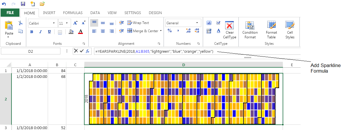

The files used in this example are available here: YearSparkFiles. You can see examples for Spread.Sheets and a list of the many features at http://spread.grapecity.com/spreadjs/sheets/.

MESCIUS inc.