This function allows users to filter a cell range on the basis of the defined criteria. The Filter operation can be performed based on a single criterion or multiple criteria.
In order to combine two or more filter conditions, users can use the " * " operator and the "+" operator. The * operator will multiply two sets of conditions in order to join the filter criteria with AND logic [when both the filter conditions have to be TRUE]. The + operator will simply join the two sets of conditions with OR logic [when one filter condition can be TRUE and the other can be FALSE].
FILTER(array,include,[if_empty])
FILTER function has the following arguments:
| Argument | Description |
|---|---|
| array | [required] Specifies the range or array that you want to filter. |
| include | [required] Specifies the filter condition expressed using an intersecting sub-range and conditional expressions. |
| if_empty | [optional] Specifies the optional value that users want to return when the filter result is empty. If value is not specified for this parameter, then #CALC! error is thrown. |
Accepts a cell range or an array of data that you want to filter. Returns a filtered array.
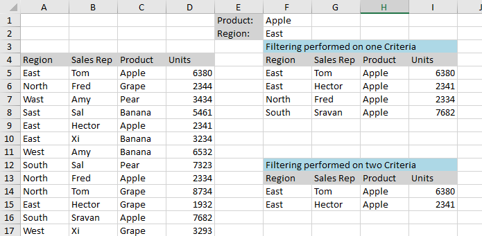
For instance - The cell F5 in the following image contains the formula "=FILTER(A5:D17, C5:C17=F1)". This formula filters the cell range A5 to D17 based on one filter criteria (when the cell range C5 to C17 matches the Product value in cell F1 i.e. Apple). As a result, all the values in the cell range A5 to D17 containing product as "Apple" will be displayed.
In another example, the cell F14 in the following image contains the formula "=FILTER(A5:D17, (C5:C17=F1)*(A5:A17=F2))". This formula filters the cell range A5 to D17 based on two filter conditions that are specified by the multiplication (*) operator. The first condition is the cell range C5 to C17 should match the Product value in cell F1 i.e. Apple and the second condition is the cell range A5 to A17 should match the region "East". As a result, all the values in the cell range A5 to D17 containing Product as "Apple" and Region as "East" will be displayed.
This function is available in Spread for Windows Forms 12.1 or later.