LET | Spread.NET 17 Formula Reference

LET

In This Topic

LET function is used to assign names to calculation results. You can also use variable names to define intermediate calculations, values, or names within the parenthesis "()" of the LET function. You need to define name and value pairs associated with the function and a calculation that uses them all.

By using this function, you don't have to remember what a specific range or cell reference refers to, or what the calculation is supposed to do, or even copy pasting the same expression all over again.

Performance Improvement Using LET Function

LET function improves the calculation performance by eliminating redundant recalculation of the intermediate values defined in the variables.

The below example shows the performance improvement by using LET function to calculate a dynamic array value and then repeatedly refers that array in a formula.

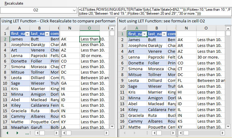
Here, both spreadsheet controls are initialized with the same list of 500 names and addresses, and both use the same formula in cell N2 to return a sorted list of unique states in a dynamic array:

=SORT(UNIQUE(Table1[state]))

The spreadsheet controls use the formula in cells O2:O48 to calculate the number of rows in the table and return a string value based on the number of rows in nested IF functions.

The left spreadsheet uses the LET function to optimize this calculation and reuse the dynamic array result inside the IF functions:

 =LET(cities,ROWS(UNIQUE(FILTER(Table1[city],Table1[state]=$N2,""))),IF(cities<10,"Less than 10.",IF(cities<20,"Between 10 and
19.",IF(cities<30,"Between 20 and 29","30 or more."))))

Whereas, the right spreadsheet does not use the LET function, and instead repeats the expression for cities inside the IF function:

=IF(ROWS(UNIQUE(FILTER(Table1[city],Table1[state]=$N2,"")))<10,"Less than
10.",IF(ROWS(UNIQUE(FILTER(Table1[city],Table1[state]=$N2,"")))<20,"Between 10 and
19.",IF(ROWS(UNIQUE(FILTER(Table1[city],Table1[state]=$N2,"")))<30,"Between 20 and 29","30 or more.")))

When the Recalculate menu item is activated to recalculate the spreadsheets, special code is used to disable CalculationOnDemand in the CalculationEngine to force all cells to recalculate, and the results are shown in the TitleInfo across the top of each spreadsheet control.

The left spreadsheet using the LET function calculates 2-4 times faster than the right spreadsheet which does not use LET function.

Syntax

LET(name1, value1, [name2…], [value2…], calculation)

Arguments

This function has these arguments:

Argument	Description
name1	First name to assign. Must begin with a letter.
value1	The value or calculation that is assigned to name1.
name2	[Optional] A second name to be assigned to a second value. If a name2 is specified, value2 and calculation becomes a required argument.
value2	[Optional] The value or calculation that is assigned to name2.
calculation	The final calculation that uses all names within the LET function. This must be the last argument of this function.

Remarks

The last argument must be a calculation that returns a result.

Data Types

Returns a Variant type.

Examples

The following sample code show the basic usage with two LET functions.

JavaScript	Copy Code
// Dynamic array - LET function requests dynamic array feature and hence we should enable it from CalcEngine before setting the formula fpSpread1.AsWorkbook().WorkbookSet.CalculationEngine.CalcFeatures \|= CalcFeatures.DynamicArray; // Set Value for (int i = 0; i < 5; i++) { fpSpread1.AsWorkbook().Worksheets[0].Cells[i, 2, 4, 2].Value = new Random(2).Next(20, 50); fpSpread1.AsWorkbook().Worksheets[0].Cells[i, 3, 4, 3].Value = new Random(3).Next(10, 40); } // set text for column header cells fpSpread1.AsWorkbook().ActiveSheet.ColumnHeader.Cells[0, 1].Text = "LET function in cell B1"; fpSpread1.AsWorkbook().ActiveSheet.ColumnHeader.Cells[0, 4].Text = "LET function in cell E1"; // set value in cell Range A1:A5 fpSpread1.AsWorkbook().Worksheets[0].Cells["A1:A5"].Value = 14; // set formula in cell B1 which will work as dynamic array fpSpread1.AsWorkbook().Worksheets[0].Cells["B1"].Formula2 = "LET(range, A1:A5, range+1)"; // LET function with two variables "range" and "const" // "range" is referring to "D1:D5" && "const" is referring to "C1:C5" fpSpread1.AsWorkbook().Worksheets[0].Cells["E1"].Formula2 = "LET(range, D1:D5, const, C1:C5, range + const)"; // set column width fpSpread1.AsWorkbook().ActiveSheet.Columns[1].ColumnWidth = 180; fpSpread1.AsWorkbook().ActiveSheet.Columns[4].ColumnWidth = 180;

JavaScript

Copy Code

  // Dynamic array - LET function requests dynamic array feature and hence we should enable it from CalcEngine before setting the formula
   fpSpread1.AsWorkbook().WorkbookSet.CalculationEngine.CalcFeatures |= CalcFeatures.DynamicArray;

  // Set Value
  for (int i = 0; i < 5; i++)
      {
        fpSpread1.AsWorkbook().Worksheets[0].Cells[i, 2, 4, 2].Value = new Random(2).Next(20, 50);
        fpSpread1.AsWorkbook().Worksheets[0].Cells[i, 3, 4, 3].Value = new Random(3).Next(10, 40);
       }
  // set text for column header cells
   fpSpread1.AsWorkbook().ActiveSheet.ColumnHeader.Cells[0, 1].Text = "LET function in cell B1";
   fpSpread1.AsWorkbook().ActiveSheet.ColumnHeader.Cells[0, 4].Text = "LET function in cell E1";

  // set value in cell Range A1:A5
   fpSpread1.AsWorkbook().Worksheets[0].Cells["A1:A5"].Value = 14;
  // set formula in cell B1 which will work as dynamic array
   fpSpread1.AsWorkbook().Worksheets[0].Cells["B1"].Formula2 = "LET(range, A1:A5, range+1)";


  // LET function with two variables "range" and "const"
  // "range" is referring to "D1:D5" && "const" is referring to "C1:C5"
  fpSpread1.AsWorkbook().Worksheets[0].Cells["E1"].Formula2 = "LET(range, D1:D5, const, C1:C5, range + const)";

  // set column width
  fpSpread1.AsWorkbook().ActiveSheet.Columns[1].ColumnWidth = 180;
  fpSpread1.AsWorkbook().ActiveSheet.Columns[4].ColumnWidth = 180;

The output of above code is shown as below where cell B1 contains the formula "= LET (range, A1: A5, range + 1)" with "range + 1" as the last argument to represent the formula that was actually evaluated. This formula returns 15 as a result.
Similarly, cell E1 contains the formula "= LET (range, D1: D5, const, C1: C5, range + const)", which uses "range" and "const" as variables. Here, "range" stands for D1: D5 and "const" stands for C1: C5. This formula returns 61 as a result.

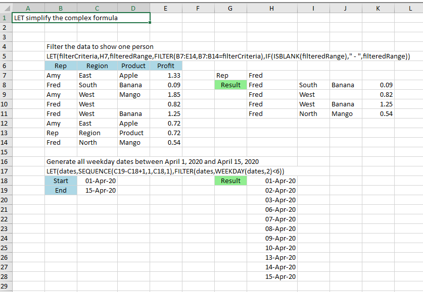
The following example considers a use case with some raw sales data which needs to be filtered to show one person and add a dash to any blank cells. This can be achieved by using the LET function to calculate the FILTER function once as shown below:

JavaScript	Copy Code
// Dynamic array - LET function requests dynamic array feature and hence we should enable it from CalcEngine before setting the formula fpSpread1.AsWorkbook().WorkbookSet.CalculationEngine.CalcFeatures \|= CalcFeatures.DynamicArray; // get the worksheet IWorksheet worksheet = fpSpread1.AsWorkbook().Worksheets[0]; // set text worksheet.Cells[0, 0].Text = "LET simplify the complex formula"; // merge cells worksheet.Cells[0, 0, 0, 3].Merge(true); worksheet.Cells[0, 0].MergePolicy = MergePolicy.Always; // set column widths fpSpread1.AsWorkbook().ActiveSheet.Columns[2].ColumnWidth = 80; fpSpread1.AsWorkbook().ActiveSheet.Columns[7].ColumnWidth = 100; // Filter the data to show one person // create formula string formula = "LET(filterCriteria,H7,filteredRange,FILTER(B7:E14,B7:B14=filterCriteria),IF(ISBLANK(filteredRange),\" - \",filteredRange))"; // set data in cells worksheet.Cells[3, 1].Text = "Filter the data to show one person"; // set formula in cells worksheet.Cells[4, 1].Text = formula; // merge cells worksheet.Cells[3, 1, 3, 4].Merge(true); worksheet.Cells[3, 1].MergePolicy = MergePolicy.Always; worksheet.Cells[4, 1, 4, 12].Merge(true); worksheet.Cells[4, 1].MergePolicy = MergePolicy.Always; // Add Data to cells worksheet.Cells[5, 1].Text = "Rep"; worksheet.Cells[5, 2].Text = "Region"; worksheet.Cells[5, 3].Text = "Product"; worksheet.Cells[5, 4].Text = "Profit"; worksheet.Cells[6, 1].Text = "Amy"; worksheet.Cells[6, 2].Text = "East"; worksheet.Cells[6, 3].Text = "Apple"; worksheet.Cells[6, 4].Value = 1.33; worksheet.Cells[7, 1].Text = "Fred"; worksheet.Cells[7, 2].Text = "South"; worksheet.Cells[7, 3].Text = "Banana"; worksheet.Cells[7, 4].Value = 0.09; worksheet.Cells[8, 1].Text = "Amy"; worksheet.Cells[8, 2].Text = "West"; worksheet.Cells[8, 3].Text = "Mango"; worksheet.Cells[8, 4].Value = 1.85; worksheet.Cells[9, 1].Text = "Fred"; worksheet.Cells[9, 2].Text = "West"; worksheet.Cells[9, 3].Text = ""; worksheet.Cells[9, 4].Value = 0.82; worksheet.Cells[10, 1].Text = "Fred"; worksheet.Cells[10, 2].Text = "West"; worksheet.Cells[10, 3].Text = "Banana"; worksheet.Cells[10, 4].Value = 1.25; worksheet.Cells[11, 1].Text = "Amy"; worksheet.Cells[11, 2].Text = "East"; worksheet.Cells[11, 3].Text = "Apple"; worksheet.Cells[11, 4].Value = 0.72; worksheet.Cells[12, 1].Text = "Rep"; worksheet.Cells[12, 2].Text = "Region"; worksheet.Cells[12, 3].Text = "Product"; worksheet.Cells[12, 4].Value = 0.72; worksheet.Cells[13, 1].Text = "Fred"; worksheet.Cells[13, 2].Text = "North"; worksheet.Cells[13, 3].Text = "Mango"; worksheet.Cells[13, 4].Value = 0.54; worksheet.Cells[6, 6].Text = "Rep"; worksheet.Cells[7, 6].Text = "Result"; worksheet.Cells[6, 7].Text = "Fred"; // set cell styling properties fpSpread1.ActiveSheet.Cells[7, 6].BackColor = System.Drawing.Color.LightGreen; fpSpread1.ActiveSheet.Cells[7, 6].HorizontalAlignment = FarPoint.Win.Spread.CellHorizontalAlignment.Center; fpSpread1.ActiveSheet.Cells[5, 1, 5, 4].BackColor = System.Drawing.Color.LightBlue; fpSpread1.ActiveSheet.Cells[5, 1, 5, 4].HorizontalAlignment = FarPoint.Win.Spread.CellHorizontalAlignment.Center; // Add dynamic array formula to cell worksheet.Cells[7, 7].Formula2 = formula; // Generate all weekday dates between 1st April and 15th April // create formula string formula1 = "LET(dates,SEQUENCE(C19-C18+1,1,C18,1),FILTER(dates,WEEKDAY(dates,2)<6))"; // create formatter string formatter = "[$-en-US]dd-mmm-yy;@"; // Add text to cell worksheet.Cells[15, 1].Text = "Generate all weekday dates between April 1, 2020 and April 15, 2020"; // set cell styling properties worksheet.Cells[15, 1, 15, 7].Merge(true); worksheet.Cells[15, 1].MergePolicy = MergePolicy.Always; // add formula to cell worksheet.Cells[16, 1].Text = formula1; // set cell styling properties worksheet.Cells[16, 1, 16, 8].Merge(true); worksheet.Cells[16, 1].MergePolicy = MergePolicy.Always; // Add text to cell worksheet.Cells[17, 1].Text = "Start"; worksheet.Cells[18, 1].Text = "End"; worksheet.Cells[17, 2].Text = new DateTime(2020, 4, 1).ToString(); worksheet.Cells[18, 2].Text = new DateTime(2020, 4, 15).ToString(); // set cell styling properties fpSpread1.ActiveSheet.Cells[17, 1, 18, 1].BackColor = System.Drawing.Color.LightBlue; fpSpread1.ActiveSheet.Cells[17, 1, 18, 1].HorizontalAlignment = FarPoint.Win.Spread.CellHorizontalAlignment.Center; // set formatter for cells worksheet.Cells[17, 2].NumberFormat = formatter; worksheet.Cells[18, 2].NumberFormat = formatter; // Add text to cell worksheet.Cells[17, 6].Text = "Result"; // set cell styling properties fpSpread1.ActiveSheet.Cells[17, 6].BackColor = System.Drawing.Color.LightGreen; fpSpread1.ActiveSheet.Cells[17, 6].HorizontalAlignment = FarPoint.Win.Spread.CellHorizontalAlignment.Center; // Add dynamic array formula to cell worksheet.Cells[17, 7].Formula2 = formula1; // set cell formatter for (var i = 0; i < 11; i++) { worksheet.Cells[i + 17, 7].NumberFormat = formatter; }

JavaScript

Copy Code

  // Dynamic array - LET function requests dynamic array feature and hence we should enable it from CalcEngine before setting the formula
 fpSpread1.AsWorkbook().WorkbookSet.CalculationEngine.CalcFeatures |= CalcFeatures.DynamicArray;
 // get the worksheet
 IWorksheet worksheet = fpSpread1.AsWorkbook().Worksheets[0];
 // set text
 worksheet.Cells[0, 0].Text = "LET simplify the complex formula";
 // merge cells
 worksheet.Cells[0, 0, 0, 3].Merge(true);
 worksheet.Cells[0, 0].MergePolicy = MergePolicy.Always;
 // set column widths
 fpSpread1.AsWorkbook().ActiveSheet.Columns[2].ColumnWidth = 80;
 fpSpread1.AsWorkbook().ActiveSheet.Columns[7].ColumnWidth = 100;

 // Filter the data to show one person
 // create formula
 string formula = "LET(filterCriteria,H7,filteredRange,FILTER(B7:E14,B7:B14=filterCriteria),IF(ISBLANK(filteredRange),\" - \",filteredRange))";
 // set data in cells
 worksheet.Cells[3, 1].Text = "Filter the data to show one person";
 // set formula in cells
 worksheet.Cells[4, 1].Text = formula;
 // merge cells
 worksheet.Cells[3, 1, 3, 4].Merge(true);
 worksheet.Cells[3, 1].MergePolicy = MergePolicy.Always;
 worksheet.Cells[4, 1, 4, 12].Merge(true);
 worksheet.Cells[4, 1].MergePolicy = MergePolicy.Always;

 // Add Data to cells
 worksheet.Cells[5, 1].Text = "Rep";
 worksheet.Cells[5, 2].Text = "Region";
 worksheet.Cells[5, 3].Text = "Product";
 worksheet.Cells[5, 4].Text = "Profit";

 worksheet.Cells[6, 1].Text = "Amy";
 worksheet.Cells[6, 2].Text = "East";
 worksheet.Cells[6, 3].Text = "Apple";
 worksheet.Cells[6, 4].Value = 1.33;

 worksheet.Cells[7, 1].Text = "Fred";
 worksheet.Cells[7, 2].Text = "South";
 worksheet.Cells[7, 3].Text = "Banana";
 worksheet.Cells[7, 4].Value = 0.09;

 worksheet.Cells[8, 1].Text = "Amy";
 worksheet.Cells[8, 2].Text = "West";
 worksheet.Cells[8, 3].Text = "Mango";
 worksheet.Cells[8, 4].Value = 1.85;

 worksheet.Cells[9, 1].Text = "Fred";
 worksheet.Cells[9, 2].Text = "West";
 worksheet.Cells[9, 3].Text = "";
 worksheet.Cells[9, 4].Value = 0.82;

 worksheet.Cells[10, 1].Text = "Fred";
 worksheet.Cells[10, 2].Text = "West";
 worksheet.Cells[10, 3].Text = "Banana";
 worksheet.Cells[10, 4].Value = 1.25;

 worksheet.Cells[11, 1].Text = "Amy";
 worksheet.Cells[11, 2].Text = "East";
 worksheet.Cells[11, 3].Text = "Apple";
 worksheet.Cells[11, 4].Value = 0.72;


 worksheet.Cells[12, 1].Text = "Rep";
 worksheet.Cells[12, 2].Text = "Region";
 worksheet.Cells[12, 3].Text = "Product";
 worksheet.Cells[12, 4].Value = 0.72;

 worksheet.Cells[13, 1].Text = "Fred";
 worksheet.Cells[13, 2].Text = "North";
 worksheet.Cells[13, 3].Text = "Mango";
 worksheet.Cells[13, 4].Value = 0.54;

 worksheet.Cells[6, 6].Text = "Rep";
 worksheet.Cells[7, 6].Text = "Result";
 worksheet.Cells[6, 7].Text = "Fred";
 // set cell styling properties
 fpSpread1.ActiveSheet.Cells[7, 6].BackColor = System.Drawing.Color.LightGreen;
 fpSpread1.ActiveSheet.Cells[7, 6].HorizontalAlignment = FarPoint.Win.Spread.CellHorizontalAlignment.Center;
 fpSpread1.ActiveSheet.Cells[5, 1, 5, 4].BackColor = System.Drawing.Color.LightBlue;
 fpSpread1.ActiveSheet.Cells[5, 1, 5, 4].HorizontalAlignment = FarPoint.Win.Spread.CellHorizontalAlignment.Center;

 // Add dynamic array formula to cell
 worksheet.Cells[7, 7].Formula2 = formula;

 // Generate all weekday dates between 1st April and 15th April
 // create formula
 string formula1 = "LET(dates,SEQUENCE(C19-C18+1,1,C18,1),FILTER(dates,WEEKDAY(dates,2)<6))";
 // create formatter 
 string formatter = "[$-en-US]dd-mmm-yy;@";
 // Add text to cell
 worksheet.Cells[15, 1].Text = "Generate all weekday dates between April 1, 2020 and April 15, 2020";
 // set cell styling properties
 worksheet.Cells[15, 1, 15, 7].Merge(true);
 worksheet.Cells[15, 1].MergePolicy = MergePolicy.Always;
 // add formula to cell
 worksheet.Cells[16, 1].Text = formula1;
 // set cell styling properties
 worksheet.Cells[16, 1, 16, 8].Merge(true);
 worksheet.Cells[16, 1].MergePolicy = MergePolicy.Always;
 // Add text to cell
 worksheet.Cells[17, 1].Text = "Start";
 worksheet.Cells[18, 1].Text = "End";
 worksheet.Cells[17, 2].Text = new DateTime(2020, 4, 1).ToString();
 worksheet.Cells[18, 2].Text = new DateTime(2020, 4, 15).ToString();
 // set cell styling properties
 fpSpread1.ActiveSheet.Cells[17, 1, 18, 1].BackColor = System.Drawing.Color.LightBlue;
 fpSpread1.ActiveSheet.Cells[17, 1, 18, 1].HorizontalAlignment = FarPoint.Win.Spread.CellHorizontalAlignment.Center;
 // set formatter for cells
 worksheet.Cells[17, 2].NumberFormat = formatter;
 worksheet.Cells[18, 2].NumberFormat = formatter;
 // Add text to cell
 worksheet.Cells[17, 6].Text = "Result";
 // set cell styling properties
 fpSpread1.ActiveSheet.Cells[17, 6].BackColor = System.Drawing.Color.LightGreen;
 fpSpread1.ActiveSheet.Cells[17, 6].HorizontalAlignment = FarPoint.Win.Spread.CellHorizontalAlignment.Center;
 // Add dynamic array formula to cell
 worksheet.Cells[17, 7].Formula2 = formula1;
 // set cell formatter
 for (var i = 0; i < 11; i++)
 {
     worksheet.Cells[i + 17, 7].NumberFormat = formatter;
 }

The output of above code will look like below:

Version Available

This function is available in Spread for Windows Forms 14.0 or later.