Spread for WinForms provides extensive support for using dynamic array formulas in the spreadsheets. When a cell contains a dynamic array formula, multiple values are returned because the elements of the array spill into the adjacent empty cells. Unlike generic arrays, dynamic arrays automatically resize when the data is inserted or removed from the source range.
The aim of introducing dynamic array formulas is to gradually replace generic array formulas that were entered previously using Ctrl+Shift+Enter (CSE). Earlier, working with formulas in spreadsheets was an extremely cumbersome and time-consuming task because users need to copy the formulas to every cell manually where they want the result to be calculated. But with the introduction of Dynamic Array Formulas, multiple results are returned as output via automatic spilling and spanning to the cell range. This reduces the overall overhead to a great extent and makes it much easier and quicker to work with array formulas in the spreadsheets.
Dynamic arrays are useful especially when you're looking for good locality of reference and want to implement effective data cache utilization in the spreadsheets. Further, they also facilitate random access with low memory footprints (in terms of compactness). Generally, this is possible because dynamic arrays have only a small fixed additional overhead for storing information about the size and capacity. Hence, dynamic arrays work wonders as a powerful tool for building cache-friendly data structures while working with spreadsheets.
Dynamic array formulas that return more than one result and spill successfully to the nearby cells are known as Spilled array formulas. Note that Spilled array formulas are not supported in Tables. However, while working with dynamic array formulas that spill to several rows and columns, the cell ranges used in the spreadsheets can be formatted explicitly to appear like tables.
A range containing the results of dynamic array formulas spanned over multiple cells is called a Spilled range. Using the HasSpill property of IRange Interface, you can check whether a cell or a range has a spilled cell within it. It returns True if all the cells in the range are part of a spilled range, False if none of the cells in the range are part of a spilled range, and null, otherwise.
When you select any cell in the range of the generated Spilled array, the entire range is highlighted with a blue color border by default. However, you can hide this blue border by setting the DynamicArrayRenderer and DynamicArrayErrorRenderer properties of the ISelectionRenderer interface to null.
The following example code hides the border of a spilled dynamic array.
| C# |
Copy Code
|
|---|---|
fpSpread1.AsWorkbook().WorkbookSet.CalculationEngine.CalcFeatures = CalcFeatures.All; IWorksheet TestActiveSheet = fpSpread1.AsWorkbook().ActiveSheet; SpreadSkin spreadSkin = fpSpread1.DefaultSkin; spreadSkin.DynamicArrayRenderer = null; spreadSkin.DynamicArrayErrorRenderer = null; TestActiveSheet.Cells["C1"].Formula2 = "A1:A4"; TestActiveSheet.Cells["C1"].Select(); |
|
| VB |
Copy Code
|
|---|---|
fpSpread1.AsWorkbook().WorkbookSet.CalculationEngine.CalcFeatures = CalcFeatures.All Dim TestActiveSheet As IWorksheet = fpSpread1.AsWorkbook().ActiveSheet Dim spreadSkin As SpreadSkin = fpSpread1.DefaultSkin spreadSkin.DynamicArrayRenderer = Nothing spreadSkin.DynamicArrayErrorRenderer = Nothing TestActiveSheet.Cells("C1").Formula2 = "A1:A4" TestActiveSheet.Cells("C1").Select() |
|
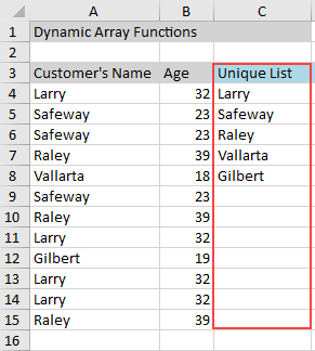
The Unique function returns a list of all the unique values in a cell range.
For instance - The cell C4 in the following image contains the formula "=UNIQUE(A4:A15)" and returns only the unique customer names from the values in cell range A4 to A15. Based on the number of unique values, the dynamic array formula spills to the cell range C5 to C8 automatically.
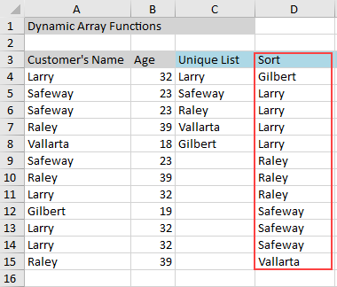
The SORT function sorts the data in a cell range or an array. The results of this function spill into the resultant range with a dynamic array of values arranged in the ascending (increasing) or descending (decreasing) order. If the sort order is not specified, then by default, the values are sorted alphabetically in the ascending order.
For instance - The cell D4 in the following image contains the formula "=SORT(A4:A15)" and returns the customer names sorted in the increasing order.
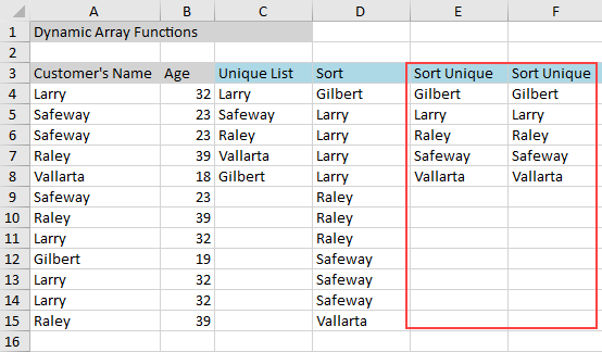
In case you want to sort all the unique values in the range A4 to A15, you can either apply the sort function on the unique list displayed in the column C4 or you can also combine both the functions SORT and UNIQUE into a single formula.
For instance, the cell E4 in the following image contains the formula "=SORT(C4#)" where # indicates a list. This formula will sort the list of values in column C (where cell C4 already contains the UNIQUE formula "=UNIQUE(A4:A15)") and displays the results in column E.
Alternatively, you can also combine both the functions SORT and UNIQUE. For instance, the cell F4 in the following image contains the formula "=SORT(UNIQUE(A4:A15))" which returns all the unique values in the range A4:A15 sorted alphabetically.
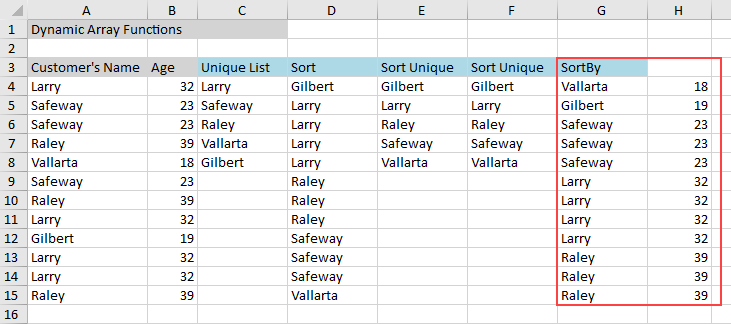
The SORTBY function sorts the contents of a cell range or an array on the basis of the values present in a corresponding range or array.
For instance - The cell G4 in the following image contains the formula "=SORTBY(A4:B15,B4:B15)". This function sorts the cell range A4 to B15 based on another cell range B4 to B15 and returns the customer names displayed along with their ages sorted in the increasing order.
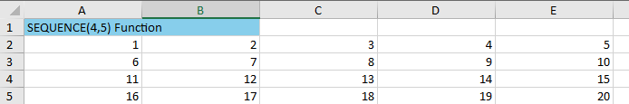
The SEQUENCE function returns a list of sequential numbers in an array in the ascending order.
For instance - The cell A2 in the following image contains the formula "=SEQUENCE(4,5)" and returns an array with values spilled to a cell range containing four rows and five columns displaying numbers in the sequence 1, 2, 3, 4 upto 20.
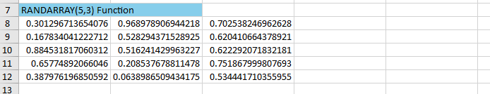
The RANDARRAY function returns an array of random numeric values. Users can specify the number of rows and columns, minimum and maximum values and indicate whether to return integers or decimal values.
For instance - The cell A8 in the following image contains the formula "=RANDARRAY(5,3)" and returns a random set of values between 0 and 1.
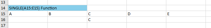
The SINGLE function returns a single value, a single cell range or an error using the implicit intersection logic.
For instance - The cell A15 in the following image contains the formula "=SINGLE(A15:E15)" and returns the result "C" in the cell C16 by evaluating the intersection of the rows and columns in the cell range A15 to E15.
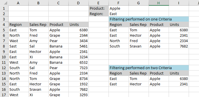
The FILTER function allows users to filter a cell range on the basis of the defined criteria. The Filter operation can be performed based on a single criterion or multiple criteria. In order to combine two or more filter conditions, users can use the " * " operator.
For instance - The cell F5 in the following image contains the formula "=FILTER(A5:D17, C5:C17=F1)". This formula filters the cell range A5 to D17 based on one filter criteria (when the cell range C5 to C17 matches the Product value in cell F1 i.e. Apple). As a result, all the values in the cell range A5 to D17 containing product as "Apple" will be displayed.
In another example, the cell F14 in the following image contains the formula "=FILTER(A5:D17, (C5:C17=F1)*(A5:A17=F2))". This formula filters the cell range A5 to D17 based on two filter conditions that are specified by the multiplication (*) operator. The first condition is the cell range C5 to C17 should match the Product value in cell F1 i.e. Apple and the second condition is the cell range A5 to A17 should match the region "East". As a result, all the values in the cell range A5 to D17 containing Product as "Apple" and Region as "East" will be displayed.
The following example code demonstrates how the dynamic array functions are used in the spreadsheet.
| C# |
Copy Code
|
|---|---|
// For enabling Dynamic Array, you need to set CalcFeatures enumeration to DynamicArray fpSpread1.AsWorkbook().WorkbookSet.CalculationEngine.CalcFeatures |= CalcFeatures.DynamicArray; fpSpread1.Sheets[0].FrozenRowCount = 1; fpSpread1.Sheets[0].Cells[0, 0].Text = "Dynamic Array Functions"; fpSpread1.Sheets[0].Cells[0, 0].BackColor = System.Drawing.Color.LightGray; fpSpread1.Sheets[0].AddSpanCell(0, 0, 1, 3); // Setting Data in Cells of Sheet[0] fpSpread1.Sheets[0].Cells[2, 0].Text = "Customer's Name"; fpSpread1.Sheets[0].Cells[2, 0].BackColor = System.Drawing.Color.LightGray; fpSpread1.Sheets[0].Cells[3, 0].Text = "Larry"; fpSpread1.Sheets[0].Cells[4, 0].Text = "Safeway"; fpSpread1.Sheets[0].Cells[5, 0].Text = "Safeway"; fpSpread1.Sheets[0].Cells[6, 0].Text = "Raley"; fpSpread1.Sheets[0].Cells[7, 0].Text = "Vallarta"; fpSpread1.Sheets[0].Cells[8, 0].Text = "Safeway"; fpSpread1.Sheets[0].Cells[9, 0].Text = "Raley"; fpSpread1.Sheets[0].Cells[10, 0].Text = "Larry"; fpSpread1.Sheets[0].Cells[11, 0].Text = "Gilbert"; fpSpread1.Sheets[0].Cells[12, 0].Text = "Larry"; fpSpread1.Sheets[0].Cells[13, 0].Text = "Larry"; fpSpread1.Sheets[0].Cells[14, 0].Text = "Raley"; fpSpread1.Sheets[0].Columns[0].Width = 120; fpSpread1.Sheets[0].Cells[2, 1].Text = "Age"; fpSpread1.Sheets[0].Cells[2, 1].BackColor = System.Drawing.Color.LightGray; fpSpread1.Sheets[0].Cells[3, 1].Text = "32"; fpSpread1.Sheets[0].Cells[4, 1].Text = "23"; fpSpread1.Sheets[0].Cells[5, 1].Text = "23"; fpSpread1.Sheets[0].Cells[6, 1].Text = "39"; fpSpread1.Sheets[0].Cells[7, 1].Text = "18"; fpSpread1.Sheets[0].Cells[8, 1].Text = "23"; fpSpread1.Sheets[0].Cells[9, 1].Text = "39"; fpSpread1.Sheets[0].Cells[10, 1].Text = "32"; fpSpread1.Sheets[0].Cells[11, 1].Text = "19"; fpSpread1.Sheets[0].Cells[12, 1].Text = "32"; fpSpread1.Sheets[0].Cells[13, 1].Text = "32"; fpSpread1.Sheets[0].Cells[14, 1].Text = "39"; fpSpread1.Sheets[0].Columns[1].Width = 50; // Setting "Unique" Formula fpSpread1.Sheets[0].Cells[2, 2].Text = "Unique List"; fpSpread1.Sheets[0].Cells[2, 2].BackColor = System.Drawing.Color.LightBlue; fpSpread1.Sheets[0].Cells[3, 2].Formula = "UNIQUE(A4:A15)"; fpSpread1.Sheets[0].Columns[2].Width = 90; // Setting "Sort" Formula fpSpread1.Sheets[0].Cells[2, 3].Text = "Sort"; fpSpread1.Sheets[0].Cells[2, 3].BackColor = System.Drawing.Color.LightBlue; fpSpread1.Sheets[0].Cells[3, 3].Formula = "SORT(A4:A15)"; fpSpread1.Sheets[0].Columns[3].Width = 90; // Setting "Sort" Formula for Unique list fpSpread1.Sheets[0].Cells[2, 4].Text = "Sort Unique"; fpSpread1.Sheets[0].Cells[2, 4].BackColor = System.Drawing.Color.LightBlue; fpSpread1.Sheets[0].Cells[3, 4].Formula = "SORT(C4#)"; fpSpread1.Sheets[0].Columns[4].Width = 90; // Setting "Sort+Unique" Formula together fpSpread1.Sheets[0].Cells[2, 5].Text = "Sort Unique"; fpSpread1.Sheets[0].Cells[2, 5].BackColor = System.Drawing.Color.LightBlue; fpSpread1.Sheets[0].Cells[3, 5].Formula = "SORT(UNIQUE(A4:A15))"; fpSpread1.Sheets[0].Columns[5].Width = 90; // Setting "SortBy" Formula wherein we sort Range A4:B15 based on the values in a corresponding range B4:B15 fpSpread1.Sheets[0].Cells[2, 6].Text = "SortBy"; fpSpread1.Sheets[0].Cells[2, 6].BackColor = System.Drawing.Color.LightBlue; fpSpread1.Sheets[0].Cells[3, 6].Formula = "SORTBY(A4:B15, B4:B15)"; fpSpread1.Sheets[0].Columns[6].Width = 90; // Setting Data in Cells of Sheet[1] fpSpread1.Sheets[1].Columns[0, 9].Width = 70; fpSpread1.Sheets[1].Cells[3, 0].Text = "Region"; fpSpread1.Sheets[1].Cells[3, 0].BackColor = System.Drawing.Color.LightGray; fpSpread1.Sheets[1].Cells[4, 0].Text = "East"; fpSpread1.Sheets[1].Cells[5, 0].Text = "North"; fpSpread1.Sheets[1].Cells[6, 0].Text = "Wast"; fpSpread1.Sheets[1].Cells[7, 0].Text = "Sast"; fpSpread1.Sheets[1].Cells[8, 0].Text = "East"; fpSpread1.Sheets[1].Cells[9, 0].Text = "East"; fpSpread1.Sheets[1].Cells[10, 0].Text = "West"; fpSpread1.Sheets[1].Cells[11, 0].Text = "South"; fpSpread1.Sheets[1].Cells[12, 0].Text = "North"; fpSpread1.Sheets[1].Cells[13, 0].Text = "North"; fpSpread1.Sheets[1].Cells[14, 0].Text = "East"; fpSpread1.Sheets[1].Cells[15, 0].Text = "South"; fpSpread1.Sheets[1].Cells[16, 0].Text = "West"; fpSpread1.Sheets[1].Cells[3, 1].Text = "Sales Rep"; fpSpread1.Sheets[1].Cells[3, 1].BackColor = System.Drawing.Color.LightGray; fpSpread1.Sheets[1].Cells[4, 1].Text = "Tom"; fpSpread1.Sheets[1].Cells[5, 1].Text = "Fred"; fpSpread1.Sheets[1].Cells[6, 1].Text = "Amy"; fpSpread1.Sheets[1].Cells[7, 1].Text = "Sal"; fpSpread1.Sheets[1].Cells[8, 1].Text = "Hector"; fpSpread1.Sheets[1].Cells[9, 1].Text = "Xi"; fpSpread1.Sheets[1].Cells[10, 1].Text = "Amy"; fpSpread1.Sheets[1].Cells[11, 1].Text = "Sal"; fpSpread1.Sheets[1].Cells[12, 1].Text = "Fred"; fpSpread1.Sheets[1].Cells[13, 1].Text = "Tom"; fpSpread1.Sheets[1].Cells[14, 1].Text = "Hector"; fpSpread1.Sheets[1].Cells[15, 1].Text = "Sravan"; fpSpread1.Sheets[1].Cells[16, 1].Text = "Xi"; fpSpread1.Sheets[1].Cells[3, 2].Text = "Product"; fpSpread1.Sheets[1].Cells[3, 2].BackColor = System.Drawing.Color.LightGray; fpSpread1.Sheets[1].Cells[4, 2].Text = "Apple"; fpSpread1.Sheets[1].Cells[5, 2].Text = "Grape"; fpSpread1.Sheets[1].Cells[6, 2].Text = "Pear"; fpSpread1.Sheets[1].Cells[7, 2].Text = "Banana"; fpSpread1.Sheets[1].Cells[8, 2].Text = "Apple"; fpSpread1.Sheets[1].Cells[9, 2].Text = "Banana"; fpSpread1.Sheets[1].Cells[10, 2].Text = "Banana"; fpSpread1.Sheets[1].Cells[11, 2].Text = "Pear"; fpSpread1.Sheets[1].Cells[12, 2].Text = "Apple"; fpSpread1.Sheets[1].Cells[13, 2].Text = "Grape"; fpSpread1.Sheets[1].Cells[14, 2].Text = "Grape"; fpSpread1.Sheets[1].Cells[15, 2].Text = "Apple"; fpSpread1.Sheets[1].Cells[16, 2].Text = "Grape"; fpSpread1.Sheets[1].Cells[3, 3].Text = "Units"; fpSpread1.Sheets[1].Cells[3, 3].BackColor = System.Drawing.Color.LightGray; fpSpread1.Sheets[1].Cells[4, 3].Text = "6380"; fpSpread1.Sheets[1].Cells[5, 3].Text = "2344"; fpSpread1.Sheets[1].Cells[6, 3].Text = "3434"; fpSpread1.Sheets[1].Cells[7, 3].Text = "5461"; fpSpread1.Sheets[1].Cells[8, 3].Text = "2341"; fpSpread1.Sheets[1].Cells[9, 3].Text = "3234"; fpSpread1.Sheets[1].Cells[10, 3].Text = "6532"; fpSpread1.Sheets[1].Cells[11, 3].Text = "7323"; fpSpread1.Sheets[1].Cells[12, 3].Text = "2334"; fpSpread1.Sheets[1].Cells[13, 3].Text = "8734"; fpSpread1.Sheets[1].Cells[14, 3].Text = "1932"; fpSpread1.Sheets[1].Cells[15, 3].Text = "7682"; fpSpread1.Sheets[1].Cells[16, 3].Text = "3293"; fpSpread1.Sheets[1].Cells[0, 4].Text = "Product:"; fpSpread1.Sheets[1].Cells[0, 4].BackColor = System.Drawing.Color.LightGray; fpSpread1.Sheets[1].Cells[0, 5].Text = "Apple"; fpSpread1.Sheets[1].Cells[1, 4].Text = "Region:"; fpSpread1.Sheets[1].Cells[1, 4].BackColor = System.Drawing.Color.LightGray; fpSpread1.Sheets[1].Cells[1, 5].Text = "East"; fpSpread1.Sheets[1].Cells[2, 5].Text = "Filtering performed on one Criteria"; fpSpread1.Sheets[1].Cells[2, 5].BackColor = System.Drawing.Color.LightBlue; fpSpread1.Sheets[1].AddSpanCell(2, 5, 1, 4); fpSpread1.Sheets[1].Cells[3, 5].Text = "Region"; fpSpread1.Sheets[1].Cells[3, 5].BackColor = System.Drawing.Color.LightGray; fpSpread1.Sheets[1].Cells[3, 6].Text = "Sales Rep"; fpSpread1.Sheets[1].Cells[3, 6].BackColor = System.Drawing.Color.LightGray; fpSpread1.Sheets[1].Cells[3, 7].Text = "Product"; fpSpread1.Sheets[1].Cells[3, 7].BackColor = System.Drawing.Color.LightGray; fpSpread1.Sheets[1].Cells[3, 8].Text = "Units"; fpSpread1.Sheets[1].Cells[3, 8].BackColor = System.Drawing.Color.LightGray; /* Setting "Filter" Formula( with one condition) wherein we filter range A5:D17 based upon criteria wherein range C5:C17 is equal to value in cell F1 */ fpSpread1.Sheets[1].Cells[4, 5].Formula = "FILTER(A5:D17, C5:C17=F1)"; fpSpread1.Sheets[1].Cells[12, 5].Text = "Region"; fpSpread1.Sheets[1].Cells[12, 5].BackColor = System.Drawing.Color.LightGray; fpSpread1.Sheets[1].Cells[12, 6].Text = "Sales Rep"; fpSpread1.Sheets[1].Cells[12, 6].BackColor = System.Drawing.Color.LightGray; fpSpread1.Sheets[1].Cells[12, 7].Text = "Product"; fpSpread1.Sheets[1].Cells[12, 7].BackColor = System.Drawing.Color.LightGray; fpSpread1.Sheets[1].Cells[12, 8].Text = "Units"; fpSpread1.Sheets[1].Cells[12, 8].BackColor = System.Drawing.Color.LightGray; fpSpread1.Sheets[1].Cells[11, 5].Text = "Filtering performed on two Criteria"; fpSpread1.Sheets[1].Cells[11, 5].BackColor = System.Drawing.Color.LightBlue; fpSpread1.Sheets[1].AddSpanCell(11, 5, 1, 4); /* Setting "Filter" Formula( with two conditions) wherein we filter range A5:D17 based upon criteria wherein range C5:C17 is equal to value in cell F1 and range A5:A17 is equal to value in cell F2 */ fpSpread1.Sheets[1].Cells[13, 5].Formula = "FILTER(A5:D17, (C5:C17=F1)*(A5:A17=F2))"; fpSpread1.Sheets[2].Columns[0, 7].Width = 130; // Setting "Sequence" FormulafpSpread1.Sheets[2].Columns[0, 7].Width = 130; fpSpread1.Sheets[2].Cells[0, 0].Text = "SEQUENCE(4,5) Function"; fpSpread1.Sheets[2].AddSpanCell(0, 0, 1, 2); fpSpread1.Sheets[2].Cells[0, 0].BackColor = System.Drawing.Color.SkyBlue; fpSpread1.Sheets[2].Cells[1, 0].Formula = "SEQUENCE(4,5)"; // Setting "RandArray" Formula fpSpread1.Sheets[2].Cells[6, 0].Text = "RANDARRAY(5,3) Function"; fpSpread1.Sheets[2].AddSpanCell(6, 0, 1, 2); fpSpread1.Sheets[2].Cells[6, 0].BackColor = System.Drawing.Color.SkyBlue; fpSpread1.Sheets[2].Cells[7, 0].Formula = "RANDARRAY(5,3)"; // Setting "Single" Formula fpSpread1.Sheets[2].Cells[13, 0].Text = "SINGLE(A15:E15) Function"; fpSpread1.Sheets[2].AddSpanCell(13, 0, 1, 2); fpSpread1.Sheets[2].Cells[13, 0].BackColor = System.Drawing.Color.SkyBlue; fpSpread1.Sheets[2].Cells[14, 0].Value = "A"; fpSpread1.Sheets[2].Cells[14, 1].Value = "B"; fpSpread1.Sheets[2].Cells[14, 2].Value = "C"; fpSpread1.Sheets[2].Cells[14, 3].Value = "D"; fpSpread1.Sheets[2].Cells[14, 4].Value = "E"; fpSpread1.Sheets[2].Cells[15, 2].Formula = "SINGLE(A15:E15)"; |
|
| VB |
Copy Code
|
|---|---|
' For enabling Dynamic Array, you need to set CalcFeatures enumeration to DynamicArray FpSpread1.AsWorkbook().WorkbookSet.CalculationEngine.CalcFeatures = FpSpread1.AsWorkbook().WorkbookSet.CalculationEngine.CalcFeatures Or CalcFeatures.DynamicArray FpSpread1.Sheets(0).FrozenRowCount = 1 FpSpread1.Sheets(0).Cells(0, 0).Text = "Dynamic Array Functions" FpSpread1.Sheets(0).Cells(0, 0).BackColor = System.Drawing.Color.LightGray FpSpread1.Sheets(0).AddSpanCell(0, 0, 1, 3) ' Setting Data in Cells of Sheets(0) FpSpread1.Sheets(0).Cells(2, 0).Text = "Customer's Name" FpSpread1.Sheets(0).Cells(2, 0).BackColor = System.Drawing.Color.LightGray FpSpread1.Sheets(0).Cells(3, 0).Text = "Larry" FpSpread1.Sheets(0).Cells(4, 0).Text = "Safeway" FpSpread1.Sheets(0).Cells(5, 0).Text = "Safeway" FpSpread1.Sheets(0).Cells(6, 0).Text = "Raley" FpSpread1.Sheets(0).Cells(7, 0).Text = "Vallarta" FpSpread1.Sheets(0).Cells(8, 0).Text = "Safeway" FpSpread1.Sheets(0).Cells(9, 0).Text = "Raley" FpSpread1.Sheets(0).Cells(10, 0).Text = "Larry" FpSpread1.Sheets(0).Cells(11, 0).Text = "Gilbert" FpSpread1.Sheets(0).Cells(12, 0).Text = "Larry" FpSpread1.Sheets(0).Cells(13, 0).Text = "Larry" FpSpread1.Sheets(0).Cells(14, 0).Text = "Raley" FpSpread1.Sheets(0).Columns(0).Width = 120 FpSpread1.Sheets(0).Cells(2, 1).Text = "Age" FpSpread1.Sheets(0).Cells(2, 1).BackColor = System.Drawing.Color.LightGray FpSpread1.Sheets(0).Cells(3, 1).Text = "32" FpSpread1.Sheets(0).Cells(4, 1).Text = "23" FpSpread1.Sheets(0).Cells(5, 1).Text = "23" FpSpread1.Sheets(0).Cells(6, 1).Text = "39" FpSpread1.Sheets(0).Cells(7, 1).Text = "18" FpSpread1.Sheets(0).Cells(8, 1).Text = "23" FpSpread1.Sheets(0).Cells(9, 1).Text = "39" FpSpread1.Sheets(0).Cells(10, 1).Text = "32" FpSpread1.Sheets(0).Cells(11, 1).Text = "19" FpSpread1.Sheets(0).Cells(12, 1).Text = "32" FpSpread1.Sheets(0).Cells(13, 1).Text = "32" FpSpread1.Sheets(0).Cells(14, 1).Text = "39" FpSpread1.Sheets(0).Columns(1).Width = 50 ' Setting "Unique" Formula FpSpread1.Sheets(0).Cells(2, 2).Text = "Unique List" FpSpread1.Sheets(0).Cells(2, 2).BackColor = System.Drawing.Color.LightBlue FpSpread1.Sheets(0).Cells(3, 2).Formula = "UNIQUE(A4:A15)" FpSpread1.Sheets(0).Columns(2).Width = 90 ' Using "Sort" Formula FpSpread1.Sheets(0).Cells(2, 3).Text = "Sort" FpSpread1.Sheets(0).Cells(2, 3).BackColor = System.Drawing.Color.LightBlue FpSpread1.Sheets(0).Cells(3, 3).Formula = "SORT(A4:A15)" FpSpread1.Sheets(0).Columns(3).Width = 90 ' Setting "Sort" Formula for Unique list FpSpread1.Sheets(0).Cells(2, 4).Text = "Sort Unique" FpSpread1.Sheets(0).Cells(2, 4).BackColor = System.Drawing.Color.LightBlue FpSpread1.Sheets(0).Cells(3, 4).Formula = "SORT(C4#)" FpSpread1.Sheets(0).Columns(4).Width = 90 ' Setting "Sort+Unique" Formula together FpSpread1.Sheets(0).Cells(2, 5).Text = "Sort Unique" FpSpread1.Sheets(0).Cells(2, 5).BackColor = System.Drawing.Color.LightBlue FpSpread1.Sheets(0).Cells(3, 5).Formula = "SORT(UNIQUE(A4:A15))" FpSpread1.Sheets(0).Columns(5).Width = 90 ' Setting "SortBy" Formula wherein we sort Range A4:B15 based on the values in a corresponding range B4:B15 FpSpread1.Sheets(0).Cells(2, 6).Text = "SortBy" FpSpread1.Sheets(0).Cells(2, 6).BackColor = System.Drawing.Color.LightBlue FpSpread1.Sheets(0).Cells(3, 6).Formula = "SORTBY(A4:B15, B4:B15)" FpSpread1.Sheets(0).Columns(6).Width = 90 FpSpread1.Sheets(1).Columns(0, 9).Width = 70 FpSpread1.Sheets(1).Cells(3, 0).Text = "Region" FpSpread1.Sheets(1).Cells(3, 0).BackColor = System.Drawing.Color.LightGray FpSpread1.Sheets(1).Cells(4, 0).Text = "East" FpSpread1.Sheets(1).Cells(5, 0).Text = "North" FpSpread1.Sheets(1).Cells(6, 0).Text = "Wast" FpSpread1.Sheets(1).Cells(7, 0).Text = "Sast" FpSpread1.Sheets(1).Cells(8, 0).Text = "East" FpSpread1.Sheets(1).Cells(9, 0).Text = "East" FpSpread1.Sheets(1).Cells(10, 0).Text = "West" FpSpread1.Sheets(1).Cells(11, 0).Text = "South" FpSpread1.Sheets(1).Cells(12, 0).Text = "North" FpSpread1.Sheets(1).Cells(13, 0).Text = "North" FpSpread1.Sheets(1).Cells(14, 0).Text = "East" FpSpread1.Sheets(1).Cells(15, 0).Text = "South" FpSpread1.Sheets(1).Cells(16, 0).Text = "West" FpSpread1.Sheets(1).Cells(3, 1).Text = "Sales Rep" FpSpread1.Sheets(1).Cells(3, 1).BackColor = System.Drawing.Color.LightGray FpSpread1.Sheets(1).Cells(4, 1).Text = "Tom" FpSpread1.Sheets(1).Cells(5, 1).Text = "Fred" FpSpread1.Sheets(1).Cells(6, 1).Text = "Amy" FpSpread1.Sheets(1).Cells(7, 1).Text = "Sal" FpSpread1.Sheets(1).Cells(8, 1).Text = "Hector" FpSpread1.Sheets(1).Cells(9, 1).Text = "Xi" FpSpread1.Sheets(1).Cells(10, 1).Text = "Amy" FpSpread1.Sheets(1).Cells(11, 1).Text = "Sal" FpSpread1.Sheets(1).Cells(12, 1).Text = "Fred" FpSpread1.Sheets(1).Cells(13, 1).Text = "Tom" FpSpread1.Sheets(1).Cells(14, 1).Text = "Hector" FpSpread1.Sheets(1).Cells(15, 1).Text = "Sravan" FpSpread1.Sheets(1).Cells(16, 1).Text = "Xi" FpSpread1.Sheets(1).Cells(3, 2).Text = "Product" FpSpread1.Sheets(1).Cells(3, 2).BackColor = System.Drawing.Color.LightGray FpSpread1.Sheets(1).Cells(4, 2).Text = "Apple" FpSpread1.Sheets(1).Cells(5, 2).Text = "Grape" FpSpread1.Sheets(1).Cells(6, 2).Text = "Pear" FpSpread1.Sheets(1).Cells(7, 2).Text = "Banana" FpSpread1.Sheets(1).Cells(8, 2).Text = "Apple" FpSpread1.Sheets(1).Cells(9, 2).Text = "Banana" FpSpread1.Sheets(1).Cells(10, 2).Text = "Banana" FpSpread1.Sheets(1).Cells(11, 2).Text = "Pear" FpSpread1.Sheets(1).Cells(12, 2).Text = "Apple" FpSpread1.Sheets(1).Cells(13, 2).Text = "Grape" FpSpread1.Sheets(1).Cells(14, 2).Text = "Grape" FpSpread1.Sheets(1).Cells(15, 2).Text = "Apple" FpSpread1.Sheets(1).Cells(16, 2).Text = "Grape" FpSpread1.Sheets(1).Cells(3, 3).Text = "Units" FpSpread1.Sheets(1).Cells(3, 3).BackColor = System.Drawing.Color.LightGray FpSpread1.Sheets(1).Cells(4, 3).Text = "6380" FpSpread1.Sheets(1).Cells(5, 3).Text = "2344" FpSpread1.Sheets(1).Cells(6, 3).Text = "3434" FpSpread1.Sheets(1).Cells(7, 3).Text = "5461" FpSpread1.Sheets(1).Cells(8, 3).Text = "2341" FpSpread1.Sheets(1).Cells(9, 3).Text = "3234" FpSpread1.Sheets(1).Cells(10, 3).Text = "6532" FpSpread1.Sheets(1).Cells(11, 3).Text = "7323" FpSpread1.Sheets(1).Cells(12, 3).Text = "2334" FpSpread1.Sheets(1).Cells(13, 3).Text = "8734" FpSpread1.Sheets(1).Cells(14, 3).Text = "1932" FpSpread1.Sheets(1).Cells(15, 3).Text = "7682" FpSpread1.Sheets(1).Cells(16, 3).Text = "3293" FpSpread1.Sheets(1).Cells(0, 4).Text = "Product:" FpSpread1.Sheets(1).Cells(0, 4).BackColor = System.Drawing.Color.LightGray FpSpread1.Sheets(1).Cells(0, 5).Text = "Apple" FpSpread1.Sheets(1).Cells(1, 4).Text = "Region:" FpSpread1.Sheets(1).Cells(1, 4).BackColor = System.Drawing.Color.LightGray FpSpread1.Sheets(1).Cells(1, 5).Text = "East" FpSpread1.Sheets(1).Cells(2, 5).Text = "Filtering performed on one Criteria" FpSpread1.Sheets(1).Cells(2, 5).BackColor = System.Drawing.Color.LightBlue FpSpread1.Sheets(1).AddSpanCell(2, 5, 1, 4) FpSpread1.Sheets(1).Cells(3, 5).Text = "Region" FpSpread1.Sheets(1).Cells(3, 5).BackColor = System.Drawing.Color.LightGray FpSpread1.Sheets(1).Cells(3, 6).Text = "Sales Rep" FpSpread1.Sheets(1).Cells(3, 6).BackColor = System.Drawing.Color.LightGray FpSpread1.Sheets(1).Cells(3, 7).Text = "Product" FpSpread1.Sheets(1).Cells(3, 7).BackColor = System.Drawing.Color.LightGray FpSpread1.Sheets(1).Cells(3, 8).Text = "Units" FpSpread1.Sheets(1).Cells(3, 8).BackColor = System.Drawing.Color.LightGray 'Setting "Filter" Formula( with one condition) wherein we filter range A5:D17 based upon 'criteria wherein Range C5: C17 is equal to value in cell F1 FpSpread1.Sheets(1).Cells(4, 5).Formula = "FILTER(A5:D17, C5:C17=F1)" FpSpread1.Sheets(1).Cells(12, 5).Text = "Region" FpSpread1.Sheets(1).Cells(12, 5).BackColor = System.Drawing.Color.LightGray FpSpread1.Sheets(1).Cells(12, 6).Text = "Sales Rep" FpSpread1.Sheets(1).Cells(12, 6).BackColor = System.Drawing.Color.LightGray FpSpread1.Sheets(1).Cells(12, 7).Text = "Product" FpSpread1.Sheets(1).Cells(12, 7).BackColor = System.Drawing.Color.LightGray FpSpread1.Sheets(1).Cells(12, 8).Text = "Units" FpSpread1.Sheets(1).Cells(12, 8).BackColor = System.Drawing.Color.LightGray FpSpread1.Sheets(1).Cells(11, 5).Text = "Filtering performed on two Criteria" FpSpread1.Sheets(1).Cells(11, 5).BackColor = System.Drawing.Color.LightBlue FpSpread1.Sheets(1).AddSpanCell(11, 5, 1, 4) 'Setting "Filter" Formula( with two conditions) wherein we filter range A5:D17 based upon 'criteria wherein Range C5: C17 is equal to value in cell F1 and range A5:A17 is equal to 'value in cell F2 FpSpread1.Sheets(1).Cells(13, 5).Formula = "FILTER(A5:D17, (C5:C17=F1)*(A5:A17=F2))" FpSpread1.Sheets(2).Columns(0, 7).Width = 130 ' Setting "Sequence" Formula FpSpread1.Sheets(2).Columns(0, 7).Width = 130 FpSpread1.Sheets(2).Cells(0, 0).Text = "SEQUENCE(4,5) Function" FpSpread1.Sheets(2).AddSpanCell(0, 0, 1, 2) FpSpread1.Sheets(2).Cells(0, 0).BackColor = System.Drawing.Color.SkyBlue FpSpread1.Sheets(2).Cells(1, 0).Formula = "SEQUENCE(4,5)" ' Setting "RandArray" Formula FpSpread1.Sheets(2).Cells(6, 0).Text = "RANDARRAY(5,3) Function" FpSpread1.Sheets(2).AddSpanCell(6, 0, 1, 2) FpSpread1.Sheets(2).Cells(6, 0).BackColor = System.Drawing.Color.SkyBlue FpSpread1.Sheets(2).Cells(7, 0).Formula = "RANDARRAY(5,3)" ' Setting "Single" Formula FpSpread1.Sheets(2).Cells(13, 0).Text = "SINGLE(A15:E15) Function" FpSpread1.Sheets(2).AddSpanCell(13, 0, 1, 2) FpSpread1.Sheets(2).Cells(13, 0).BackColor = System.Drawing.Color.SkyBlue FpSpread1.Sheets(2).Cells(14, 0).Value = "A" FpSpread1.Sheets(2).Cells(14, 1).Value = "B" FpSpread1.Sheets(2).Cells(14, 2).Value = "C" FpSpread1.Sheets(2).Cells(14, 3).Value = "D" FpSpread1.Sheets(2).Cells(14, 4).Value = "E" FpSpread1.Sheets(2).Cells(15, 2).Formula = "SINGLE(A15:E15)" |
|