A pareto sparkline can be used to highlight the most important items in a set of values. This sparkline usually is taken as a quality tool since it helps analyze and prioritize issue resolution.
The pareto sparkline formula have the following format:
=PARETOSPARKLINE(points, [pointIndex, colorRange, target, target2, hightlightPosition, label, vertical, targetColor, target2Color, labelColor, barSize])
The formula options are described:
| Option | Description |
| points | A reference that represents the range of cells that contains all values, such as "B2:B7". |
|
pointIndex Optional |
A number or reference that represents the segment's index of the points, such as 1 or "D2". The pointIndex is >= 1. |
|
colorRange Optional |
A reference that represents the range of cells that contain the color for the segment box, such as "D2:D7". The default value is none. |
|
target Optional |
A number or reference that represents the 'target' line position, such as 0.5. The default value is none. The target line color is #8CBF64 if shown. |
|
target2 Optional |
A number or reference that represents the 'target2' line position, such as 0.8. The default value is none. The target2 line color is #EE5D5D if shown. |
|
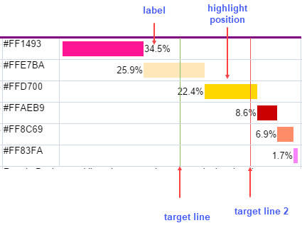
highlightPosition Optional |
A number or reference that represents the rank of the segment to be colored in red, such as 3. The default value is none. If you set the highlightPosition to a value such as 4, then the fourth segment box's color is set to #CB0000. If you do not set the highlightPosition, the segment box's color is set to the color you assigned to the colorRange or the default color #969696. |
|
label Optional |
A number that represents whether the segment's label is displayed as the cumulated percentage (label = 1) or the single percentage or none (label = 2) or none, such as 2,1. The default value is 0. |
|
vertical Optional |
A boolean that represents whether the box's direction is vertical or horizontal. The default value is False. |
|
targetColor Optional |
A color string that indicates the color of the target line. |
|
target2Color Optional |
A color string that indicates the color of the target2 line. |
|
labelColor Optional |
A color string that indicates the label fore color. |
|
barSize Optional |
A number value greater than 0 and less than or equal to 1, which indicates the percentage of bar width or height according to the cell width or height. |
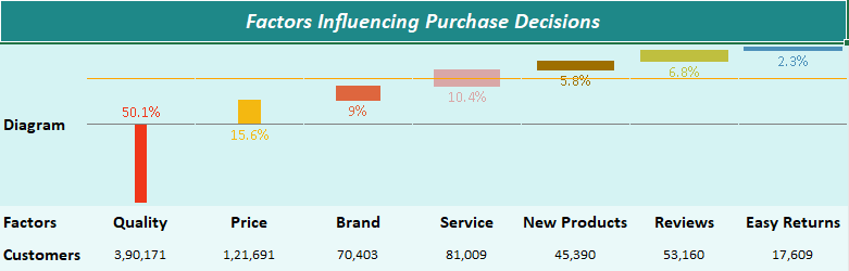
Consider a scenario where a survey is conducted on an e-commerce site to determine how a customer decides to purchase products from the site. A pareto sparkline helps highlight the most decisive factors and analyze how to benefit from the result.
| C# |
Copy Code
|
|---|---|
// Get sheet var worksheet = fpSpread1_Sheet1.AsWorksheet(); // Set data for sparkline worksheet.SetValue(2, 0, new object[,] { {"Factors","Quality","Price","Brand","Service","New Products","Reviews","Easy Returns"}, {"Customers",390171,121691,70403,81009,45390,53160,17609}, {"Color","#F0371A","#F4B811","#DE663E","#D9A7A7","#9E6F00","#BFBF3F","#4C90BA"}, {"BarSize",0.1,0.2,0.4,0.6,0.7,0.8,0.9} }); worksheet.Cells["A2"].Text = "Diagram"; // Set formula worksheet.Cells["B2"].Formula2 = "PARETOSPARKLINE(B4:H4,,B5:H5,0.5,0.8,0,2,TRUE,\"Gray\",\"Orange\",B5:H5,B6:H6)"; |
|
| Visual Basic |
Copy Code
|
|---|---|
'Get sheet Dim worksheet = FpSpread1_Sheet1.AsWorksheet() 'Set data for sparkline worksheet.SetValue(2, 0, New Object(,) { {"Factors", "Quality", "Price", "Brand", "Service", "New Products", "Reviews", "Easy Returns"}, {"Customers", 390171, 121691, 70403, 81009, 45390, 53160, 17609}, {"Color", "#F0371A", "#F4B811", "#DE663E", "#D9A7A7", "#9E6F00", "#BFBF3F", "#4C90BA"}, {"BarSize", 0.1, 0.2, 0.4, 0.6, 0.7, 0.8, 0.9} }) worksheet.Cells("A2").Text = "Diagram" 'Set formula worksheet.Cells("B2").Formula2 = "PARETOSPARKLINE(B4:H4,,B5:H5,0.5,0.8,0,2,TRUE,""Gray"",""Orange"",B5:H5,B6:H6)" |
|

You can also set additional sparkline settings in the dialog if available.