You can use this rule to highlight data that meets one of the following conditions:
After you choose one of the options above, enter a value or formula against which each cell is compared. If the cell data satisfies that criteria, then the formatting is applied.
You can select a predefined highlight style or create a custom highlight style. The following rules are highlight style rules:
This figure illustrates the following example.
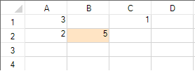
This example code creates the between values rule and uses the SetConditionalFormatting method to apply the rule.
| C# |
Copy Code
|
|---|---|
private void Form1_Load(object sender, EventArgs e) { fpSpread1.Sheets[0].Cells[0, 0].Value = 3; fpSpread1.Sheets[0].Cells[1, 0].Value = 2; fpSpread1.Sheets[0].Cells[1, 1].Value = 5; fpSpread1.Sheets[0].Cells[0, 2].Value = 1; } private void button1_Click(object sender, EventArgs e) { FarPoint.Win.Spread.BetweenValuesConditionalFormattingRule between = new FarPoint.Win.Spread.BetweenValuesConditionalFormattingRule(true, 10, false, 20, false); between.FirstValue = 10; between.SecondValue = 20; between.IsNotBetween = true; between.BackColor = Color.Bisque; fpSpread1.ActiveSheet.SetConditionalFormatting(1, 1, between); } |
|
| VB |
Copy Code
|
|---|---|
Private Sub Form1_Load(ByVal sender As System.Object, ByVal e As System.EventArgs) Handles MyBase.Load fpSpread1.Sheets(0).Cells(0, 0).Value = 3 fpSpread1.Sheets(0).Cells(1, 0).Value = 2 fpSpread1.Sheets(0).Cells(1, 1).Value = 5 fpSpread1.Sheets(0).Cells(0, 2).Value = 1 End Sub Private Sub Button1_Click(ByVal sender As System.Object, ByVal e As System.EventArgs) Handles Button1.Click Dim between As New FarPoint.Win.Spread.BetweenValuesConditionalFormattingRule(True, 10, False, 20, False) between.FirstValue = 10 between.SecondValue = 20 between.IsNotBetween = True between.BackColor = Color.Bisque fpSpread1.ActiveSheet.SetConditionalFormatting(1, 1, between) End Sub |
|