The top or bottom rules apply formatting to cells whose values fall in the top or bottom percent. The top ranked rule specifies the top or bottom values. The average rule applies to the greater or lesser average value of the entire range.
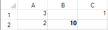
The following figure shows a top rule that sets the style for the above average value in the range of values; the code to create the example is provided in the example.
The following options are available:
This example code creates an average rule and uses the SetConditionalFormatting method to apply the rule.
| C# |
Copy Code
|
|---|---|
private void Form1_Load(object sender, EventArgs e) { fpSpread1.Sheets[0].Cells[0, 0].Value = 3; fpSpread1.Sheets[0].Cells[1, 0].Value = 2; fpSpread1.Sheets[0].Cells[1, 1].Value = 10; fpSpread1.Sheets[0].Cells[0, 2].Value = 1; } private void button1_Click(object sender, EventArgs e) { //Average CF FarPoint.Win.Spread.AverageConditionalFormattingRule average = new FarPoint.Win.Spread.AverageConditionalFormattingRule(true, true); average.IsAbove = true; average.IsIncludeEquals = true; average.StandardDeviation = 2; average.FontStyle = new FarPoint.Win.Spread.SpreadFontStyle(FarPoint.Win.Spread.RegularBoldItalicFontStyle.Bold); fpSpread1.ActiveSheet.SetConditionalFormatting(1, 1, average); } |
|
| VB |
Copy Code
|
|---|---|
Private Sub Form1_Load(ByVal sender As System.Object, ByVal e As System.EventArgs) Handles MyBase.Load fpSpread1.Sheets(0).Cells(0, 0).Value = 3 fpSpread1.Sheets(0).Cells(1, 0).Value = 2 fpSpread1.Sheets(0).Cells(1, 1).Value = 10 fpSpread1.Sheets(0).Cells(0, 2).Value = 1 End Sub Private Sub Button1_Click(ByVal sender As System.Object, ByVal e As System.EventArgs) Handles Button1.Click 'Average CF Dim average As New FarPoint.Win.Spread.AverageConditionalFormattingRule(True, True) average.IsAbove = True average.IsIncludeEquals = True average.StandardDeviation = 2 average.FontStyle = New FarPoint.Win.Spread.SpreadFontStyle(FarPoint.Win.Spread.RegularBoldItalicFontStyle.Bold) fpSpread1.ActiveSheet.SetConditionalFormatting(1, 1, average) End Sub |
|