You can set rules that display certain icons when a cell value is greater than, equal to, or less than a value.
You can use built-in icon sets for the rule. You can also specify individual icons to use in the icon set with the IconRuleSet property and the IconSetConditionalFormattingRule class. You can use custom icons with the AddIcon method and the CustomIconContainer property.
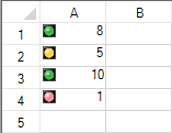
The following figure illustrates cells that display the built-in icons.
This example code creates an icon set rule and uses the SetConditionalFormatting method to apply the rule.
| C# |
Copy Code
|
|---|---|
private void Form1_Load(object sender, EventArgs e) { fpSpread1.Sheets[0].Cells[0, 0].Value = 8; fpSpread1.Sheets[0].Cells[1, 0].Value = 5; fpSpread1.Sheets[0].Cells[2, 0].Value = 10; fpSpread1.Sheets[0].Cells[3, 0].Value = 1; } private void button1_Click(object sender, EventArgs e) { FarPoint.Win.Spread.Model.CellRange celRange1 = new FarPoint.Win.Spread.Model.CellRange(0, 0, 4, 1); FarPoint.Win.Spread.IconSetConditionalFormattingRule rule = new FarPoint.Win.Spread.IconSetConditionalFormattingRule(FarPoint.Win.Spread.ConditionalFormattingIconSetStyle.ThreeRimmedTrafficLights ); fpSpread1.Sheets[0].SetConditionalFormatting(new FarPoint.Win.Spread.Model.CellRange[] { celRange1 }, rule); } |
|
| VB |
Copy Code
|
|---|---|
Private Sub Form1_Load(ByVal sender As System.Object, ByVal e As System.EventArgs) Handles MyBase.Load
        fpSpread1.Sheets(0).Cells(0, 0).Value = 8
        fpSpread1.Sheets(0).Cells(1, 0).Value = 5
        fpSpread1.Sheets(0).Cells(2, 0).Value = 10
        fpSpread1.Sheets(0).Cells(3, 0).Value = 1
    End Sub

    Private Sub Button1_Click(ByVal sender As System.Object, ByVal e As System.EventArgs) Handles Button1.Click
        Dim celRange1 As New FarPoint.Win.Spread.Model.CellRange(0, 0, 4, 1)
        Dim rule As New FarPoint.Win.Spread.IconSetConditionalFormattingRule(FarPoint.Win.Spread.ConditionalFormattingIconSetStyle.ThreeRimmedTrafficLights)
        fpSpread1.Sheets(0).SetConditionalFormatting(New FarPoint.Win.Spread.Model.CellRange() {celRange1}, rule)
      End Sub
|
|